
- –Т–Є–і–µ–Њ 195
- –Я—А–Њ—Б–Љ–Њ—В—А–Њ–≤ 850 941
Machine Learning & Simulation
–У–µ—А–Љ–∞–љ–Є—П
–Ф–Њ–±–∞–≤–ї–µ–љ 27 —Д–µ–≤ 2021
Explaining topics of рЯ§Ц Machine Learning & рЯМК Simulation with intuition, visualization and code.
------
Hey,
welcome to my channel of explanatory videos for Machine Learning & Simulation. I cover topics from Probabilistic Machine Learning, High-Performance Computing, Continuum Mechanics, Numerical Analysis, Computational Fluid Dynamics, Automatic Differentiation and Adjoint Methods. Many videos include hands-on coding parts in Python, Julia, or C++. The videos also showcase the application of the topics in modern libraries like JAX, TensorFlow Probability, NumPy, SciPy, FEniCS, PETSc and many more.
All material is also available on the GitHub Repo of the channel: github.com/Ceyron/machine-learning-and-simulation
Enjoy :) And please leave feedback.
If you liked the videos, feel free to support the channel on Patreon: www.patreon.com/MLsim
If you want to make a one-time donation, you can do so via PayPal: paypal.me/FelixMKoehler
Reverse Mode Autodiff in Python (general compute graph)
Let's implement automatic differentiation (=backpropagation) for a general directed acyclic compute graph to compute the gradient of a scalar-valued loss function. Here is the notebook: github.com/Ceyron/machine-learning-and-simulation/blob/main/english/adjoints_sensitivities_automatic_differentiation/simple_autodiff_external_static_dag.ipynb
-------
рЯСЙ This educational series is supported by the world-leaders in integrating machine learning and artificial intelligence with simulation and scientific computing, Pasteur Labs and Institute for Simulation Intelligence. Check out simulation.science/ for more on their pursuit of 'Nobel-Turing' technologies (arxiv.org/abs/2112.03235 ), and for part...
–Я—А–Њ—Б–Љ–Њ—В—А–Њ–≤: 901
–Т–Є–і–µ–Њ


Unrolled vs. Implicit Autodiff
–Я—А–Њ—Б–Љ–Њ—В—А–Њ–≤ 8252 –Љ–µ—Б—П—Ж–∞ –љ–∞–Ј–∞–і
Unrolled Differentiation of an iterative algorithm can produce the "Curse of Unrolling" phenomenon on the Jacobian suboptimality. How much better is implicit automatic differentiation? Here is the code: github.com/Ceyron/machine-learning-and-simulation/blob/main/english/adjoints_sensitivities_automatic_differentiation/curse_of_unrolling_against_implicit_diff.ipynb рЯСЙ This educational series is s...

Unrolled Autodiff of iterative Algorithms
–Я—А–Њ—Б–Љ–Њ—В—А–Њ–≤ 1,4 —В—Л—Б.2 –Љ–µ—Б—П—Ж–∞ –љ–∞–Ј–∞–і
When you have iterative parts in a computational graph (like optimization problems, linear solves, root-finding etc.) you can either unroll differentiate or implicitly differentiate them. The former has a counter-intuitive Jacobian converge (=Curse of Unrolling). Code: github.com/Ceyron/machine-learning-and-simulation/blob/main/english/adjoints_sensitivities_automatic_differentiation/curse_of_u...

UNet Tutorial in JAX
–Я—А–Њ—Б–Љ–Њ—В—А–Њ–≤ 1,4 —В—Л—Б.3 –Љ–µ—Б—П—Ж–∞ –љ–∞–Ј–∞–і
UNets are a famous architecture for image segmentation. With their hierarchical structure they have a wide receptive field. Similar to multigrid methods, we will use them in this video to solve the Poisson equation in the Equinox deep learning framework. Here is the code: github.com/Ceyron/machine-learning-and-simulation/blob/main/english/neural_operators/simple_unet_poisson_solver_in_jax.ipynb...
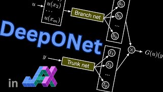
DeepONet Tutorial in JAX
–Я—А–Њ—Б–Љ–Њ—В—А–Њ–≤ 2,4 —В—Л—Б.3 –Љ–µ—Б—П—Ж–∞ –љ–∞–Ј–∞–і
Neural operators are deep learning architectures that approximate nonlinear operators, for instance, to learn the solution to a parametric PDE. The DeepONet is one type in which we can query the output at arbitrary points. Here is the code: github.com/Ceyron/machine-learning-and-simulation/blob/main/english/neural_operators/simple_deepOnet_in_JAX.ipynb рЯСЙ This educational series is supported by ...

Spectral Derivative in 3d using NumPy and the RFFT
–Я—А–Њ—Б–Љ–Њ—В—А–Њ–≤ 1,1 —В—Л—Б.4 –Љ–µ—Б—П—Ж–∞ –љ–∞–Ј–∞–і
The Fast Fourier Transform works in arbitrary dimensions. Hence, we can also use it to derive n-dimensional fields spectrally. In this video, we clarify the details of this procedure, including how to adapt the np.meshgrid indexing style. Here is the code: github.com/Ceyron/machine-learning-and-simulation/blob/main/english/fft_and_spectral_methods/spectral_derivative_3d_in_numpy_with_rfft.ipynb...

NumPy.fft.rfft2 - real-valued spectral derivatives in 2D
–Я—А–Њ—Б–Љ–Њ—В—А–Њ–≤ 5474 –Љ–µ—Б—П—Ж–∞ –љ–∞–Ј–∞–і
How does the real-valued fast Fourier transformation work in two dimensions? The Fourier shape becomes a bit tricky when only one axis is halved, requiring special care when setting up the wavenumber array. Here is the notebook: github.com/Ceyron/machine-learning-and-simulation/blob/main/english/fft_and_spectral_methods/spectral_derivative_2d_in_numpy_with_rfft.ipynb рЯСЙ This educational series i...

2D Spectral Derivatives with NumPy.FFT
–Я—А–Њ—Б–Љ–Њ—В—А–Њ–≤ 1,2 —В—Л—Б.5 –Љ–µ—Б—П—Ж–µ–≤ –љ–∞–Ј–∞–і
The Fast Fourier Transform allows to easily take derivatives of periodic functions. In this video, we look at how this concept extends to two dimensions, such as how to create the wavenumber grid and how to deal with partial derivatives. Here is the notebook: github.com/Ceyron/machine-learning-and-simulation/blob/main/english/fft_and_spectral_methods/spectral_derivative_2d_in_numpy.ipynb рЯСЙ This...

Softmax - Pullback/vJp rule
–Я—А–Њ—Б–Љ–Њ—В—А–Њ–≤ 4285 –Љ–µ—Б—П—Ж–µ–≤ –љ–∞–Ј–∞–і
The softmax is the last layer in deep networks used for classification, but how do you backpropagate over it? What primitive rule must the automatic differentiation framework understand? Here are the note: github.com/Ceyron/machine-learning-and-simulation/blob/main/english/adjoints_sensitivities_automatic_differentiation/rules/softmax_pullback.pdf рЯСЙ This educational series is supported by the w...
Softmax - Pushforward/Jvp rule
–Я—А–Њ—Б–Љ–Њ—В—А–Њ–≤ 4085 –Љ–µ—Б—П—Ж–µ–≤ –љ–∞–Ј–∞–і
The softmax is a common function in machine learning to map logit values to discrete probabilities. It is often used as the final layer in a neural network applied to multinomial regression problems. Here, we derive its rule for forward-mode AD. Here are the notes: github.com/Ceyron/machine-learning-and-simulation/blob/main/english/adjoints_sensitivities_automatic_differentiation/rules/softmax_...
Fourier Neural Operators (FNO) in JAX
–Я—А–Њ—Б–Љ–Њ—В—А–Њ–≤ 6 —В—Л—Б.6 –Љ–µ—Б—П—Ж–µ–≤ –љ–∞–Ј–∞–і
Neural Operators are mappings between (discretized) function spaces, like from the IC of a PDE to its solution at a later point in time. FNOs do so by employing a spectral convolution that allows for multiscale properties. Let's code a simple example in JAX: github.com/Ceyron/machine-learning-and-simulation/blob/main/english/neural_operators/simple_FNO_in_JAX.ipynb рЯСЙ This educational series is ...
Custom Rollout transformation in JAX (using scan)
–Я—А–Њ—Б–Љ–Њ—В—А–Њ–≤ 5617 –Љ–µ—Б—П—Ж–µ–≤ –љ–∞–Ј–∞–і
Calling a timestepper repeatedly on its own output produces a temporal trajectory. In this video, we build syntactic sugar around jax.lax.scan to get a function transformation doing exactly this very efficiently. Here is the code: github.com/Ceyron/machine-learning-and-simulation/blob/main/english/jax_tutorials/rollout_transformation.ipynb рЯСЙ This educational series is supported by the world-lea...
JAX.lax.scan tutorial (for autoregressive rollout)
–Я—А–Њ—Б–Љ–Њ—В—А–Њ–≤ 1,7 —В—Л—Б.7 –Љ–µ—Б—П—Ж–µ–≤ –љ–∞–Ј–∞–і
Do you still loop, append to a list, and stack as an array? That's the application for jax.lax.scan. With this command, producing trajectories becomes a blast. Here is the code: github.com/Ceyron/machine-learning-and-simulation/blob/main/english/jax_tutorials/jax_lax_scan_tutorial.ipynb рЯСЙ This educational series is supported by the world-leaders in integrating machine learning and artificial in...
Upgrade the KS solver in JAX to 2nd order
–Я—А–Њ—Б–Љ–Њ—В—А–Њ–≤ 7447 –Љ–µ—Б—П—Ж–µ–≤ –љ–∞–Ј–∞–і
The Exponential Time Differencing algorithm of order one applied to the Kuramoto-Sivashinsky equation quickly becomes unstable. Let's fix that by upgrading it to a Runge-Kutta-style second-order method. Here is the code: github.com/Ceyron/machine-learning-and-simulation/blob/main/english/fft_and_spectral_methods/ks_solver_etd_and_etdrk2_in_jax.ipynb рЯСЙ This educational series is supported by the...
Simple KS solver in JAX
–Я—А–Њ—Б–Љ–Њ—В—А–Њ–≤ 2 —В—Л—Б.8 –Љ–µ—Б—П—Ж–µ–≤ –љ–∞–Ј–∞–і
The Kuramoto-Sivashinsky is a fourth-order partial differential equation that shows highly chaotic dynamics. It has become an exciting testbed for deep learning methods in physics. Here, we will code a simple Exponential Time Differencing (ETD) solver in JAX/Python. Code: github.com/Ceyron/machine-learning-and-simulation/blob/main/english/fft_and_spectral_methods/ks_solver_etd_in_jax.ipynb рЯСЙ Th...
np.fft.rfft for spectral derivatives in Python
–Я—А–Њ—Б–Љ–Њ—В—А–Њ–≤ 1 —В—Л—Б.8 –Љ–µ—Б—П—Ж–µ–≤ –љ–∞–Ј–∞–і
np.fft.rfft for spectral derivatives in Python
Spectral Derivative with FFT in NumPy
–Я—А–Њ—Б–Љ–Њ—В—А–Њ–≤ 2,3 —В—Л—Б.8 –Љ–µ—Б—П—Ж–µ–≤ –љ–∞–Ј–∞–і
Spectral Derivative with FFT in NumPy
Physics-Informed Neural Networks in Julia
–Я—А–Њ—Б–Љ–Њ—В—А–Њ–≤ 3,3 —В—Л—Б.9 –Љ–µ—Б—П—Ж–µ–≤ –љ–∞–Ј–∞–і
Physics-Informed Neural Networks in Julia
Physics-Informed Neural Networks in JAX (with Equinox & Optax)
–Я—А–Њ—Б–Љ–Њ—В—А–Њ–≤ 6 —В—Л—Б.10 –Љ–µ—Б—П—Ж–µ–≤ –љ–∞–Ј–∞–і
Physics-Informed Neural Networks in JAX (with Equinox & Optax)
Neural Networks using Lux.jl and Zygote.jl Autodiff in Julia
–Я—А–Њ—Б–Љ–Њ—В—А–Њ–≤ 2,1 —В—Л—Б.11 –Љ–µ—Б—П—Ж–µ–≤ –љ–∞–Ј–∞–і
Neural Networks using Lux.jl and Zygote.jl Autodiff in Julia
Neural Networks in Equinox (JAX DL framework) with Optax
–Я—А–Њ—Б–Љ–Њ—В—А–Њ–≤ 2,5 —В—Л—Б.–У–Њ–і –љ–∞–Ј–∞–і
Neural Networks in Equinox (JAX DL framework) with Optax
Neural Networks in pure JAX (with automatic differentiation)
–Я—А–Њ—Б–Љ–Њ—В—А–Њ–≤ 2,3 —В—Л—Б.–У–Њ–і –љ–∞–Ј–∞–і
Neural Networks in pure JAX (with automatic differentiation)
Neural Network learns sine function in NumPy/Python with backprop from scratch
–Я—А–Њ—Б–Љ–Њ—В—А–Њ–≤ 1,8 —В—Л—Б.–У–Њ–і –љ–∞–Ј–∞–і
Neural Network learns sine function in NumPy/Python with backprop from scratch
Simple reverse-mode Autodiff in Python
–Я—А–Њ—Б–Љ–Њ—В—А–Њ–≤ 2,2 —В—Л—Б.–У–Њ–і –љ–∞–Ј–∞–і
Simple reverse-mode Autodiff in Python
Animating the learning process of a Neural Network
–Я—А–Њ—Б–Љ–Њ—В—А–Њ–≤ 2,3 —В—Л—Б.–У–Њ–і –љ–∞–Ј–∞–і
Animating the learning process of a Neural Network
Neural Network learns Sine Function with custom backpropagation in Julia
–Я—А–Њ—Б–Љ–Њ—В—А–Њ–≤ 1,3 —В—Л—Б.–У–Њ–і –љ–∞–Ј–∞–і
Neural Network learns Sine Function with custom backpropagation in Julia
Simple reverse-mode Autodiff in Julia - Computational Chain
–Я—А–Њ—Б–Љ–Њ—В—А–Њ–≤ 762–У–Њ–і –љ–∞–Ј–∞–і
Simple reverse-mode Autodiff in Julia - Computational Chain
Neural ODE - Pullback/vJp/adjoint rule
–Я—А–Њ—Б–Љ–Њ—В—А–Њ–≤ 1,3 —В—Л—Б.–У–Њ–і –љ–∞–Ј–∞–і
Neural ODE - Pullback/vJp/adjoint rule
Neural ODEs - Pushforward/Jvp rule
–Я—А–Њ—Б–Љ–Њ—В—А–Њ–≤ 752–У–Њ–і –љ–∞–Ј–∞–і
Neural ODEs - Pushforward/Jvp rule
L2 Loss (Least Squares) - Pullback/vJp rule
–Я—А–Њ—Б–Љ–Њ—В—А–Њ–≤ 298–У–Њ–і –љ–∞–Ј–∞–і
L2 Loss (Least Squares) - Pullback/vJp rule
Excellent.
Thanks :)
Thanks for such a informative video. I am doing multiphase flow modelling in porous media basically solving Continuity and Darcy equations for oil and water phases. So, during the calculation I ended up vector valued function ( System of Lin. Eqs. with 450 Eqs and 450 Unknowns). Ton calculate Jacobian for this function what would you recommend ? Should I use jacobian function from ForwardDiff ? Thank You.
Thank you for the kind comment :). Yes, I think that can be a good choice. For (approx.) square Jacobians, forward-mode often turns out to be the superior approach.
What program is he using
Python library: PhiFlow Editor: VS Code
It's my third day of trying to understand basics of EM and ELBO and I found this video. Now, there won't be a forth. Thankyou
That's amazing вЭ§пЄП I'm happy the video was helpful. рЯШК
Thank you so much for this tutorial Felix!
My pleasure! Thanks for the kind comment рЯШК
I have a question here. Mean Field Approach tells us how to choose the kind of surrogate posterior and eventually we will get the optimal solution for q. However, in the previous lessons, we were assuming that surrogate posterior q is distributed according to a certain distribution and then solving the problem by using maximizing the ELBO. But at that time, we didn't know which type of distribution is the most appropriate one to choose for q. This gave me the illusion that as long as the following assumption is true: surrogate posterior can be divided into smaller independent distribution, the way of maximizing the ELBO to solve the VI problem is meaningless because we can just use Mean Field Approach to solve the VI problem without choosing an arbitrary distribution of q. I am not sure if my understanding is correct.
Great video! Particularly liked the Null hypothesis demonstration in scipy :). Would love more of these coding tutorials from you, as you have a very good way of explaining things inutuively..
Thanks рЯЩП The channel has more of this kind, e.g., to write simple PDE simulations. Or do you mean more like showcasing Python libraries?
@@MachineLearningSimulation No, I was referring to the general machine learning algorithms/nerual network implementation stuff. Seems like you have a lot of videos on it, Will check them out!
@@Dhadheechi Thanks :)
I just discovered your channel and... I do not have words, unlimited thanks from France!
Thank you for this super kind comment рЯШК Welcome to the channel, glad you enjoy the autodiff content, I love creating videos on it.
Your videos are all so well explained, I would to do the same amazing work one day, thank you!
Thank you рЯШК I can only encourage you to get started, start with sth small and upload it even if you think it's not perfect yet, improvement will come over time рЯСН
i love u bro
Haha :D I'm glad the video was helpful
You saved me! I was so frustrated that I could not understand it, but you video is so clear and understandable!
Wonderful рЯСН I'm very happy рЯШК Thanks for the kind comment.
This video saved my day. Thank you so much!
You're welcome! рЯШК
Very helpful video, thank you so much рЯШК
YouвАЩre welcome рЯШК
HOW OT MAEK THING IN PYTHON: import thing; thing.do();
Thaks for sharing this useful tutorial.
You're welcome рЯ§Ч
Very interesting. If we wanted to implement for poisson on a membrane could we pretty much keep the original unet image implementation?
Thanks for the kind comment рЯШК Yes, I think that should work (given you again have homogeneous Dirichlet BCs).
I think you refer to extending the poisson emulation to 2d.
@@MachineLearningSimulation yes
@@MachineLearningSimulation maybe I need to think more carefully. What kind of shape of domain I might have would make this complicated
understood вЬЕ
4:10 why do you use dy in dL/dy instead of d(y+ef) like you do next in d(y+ef)/de in the chain rule? Isn't this supposed to be the same function that the deriavtive is taken with respect to, as the function that is differentiated with respect to to a variable?
Python is assрЯТА
bro really went" import fluidSim fluid = fluidSim.water("darkmode") fluid.start()"
Hello, teacher. Your vedios benifit me a lot пЉБAnd I have a questionпЉМIt has been bothering me for a long time. How can something be called adjoint?
You're welcome :) Thanks for the kind comment. The easiest explanation is that you can call a transposed matrix also the adjoint of that matrix.
awesome!
"fastest" "python"
Here: fasted in terms of overall productivity рЯШЙ
This is great! Working on a package that uses the adjoint method for implicit differentiation and this video explained things really well :D
You're welcome :)
oh god, thank you that was the real beset
You're welcome :)
Many thanks for the great video, I was looking for something along these lines. I have two questions. The first is regarding how you just chose that the term multiplying the Jacobian vanishes. Where do you get the freedom to impose that without this hurting the optimization procedure? From my recollection on Lagrange multipliers, we usually solve for them once we consider the variation of the Lagrangian to be zero, but we don't get much freedom - in fact, whatever they end up being may even have physical meaning, e.g. being normal forces on mechanical systems which are constrained to be on a surface. The second question regards why using Lagrange multipliers should work in the first place. I understand that, if we wanted to find saddle points for the loss then indeed this is the path; but how do we justify using a Lagrange multiplier we found during the minimization process to compute the Jacobian of solution w.r.t to parameters in general?
I was looking at the reference code that you mentioned in the jupyter notebook and found that they coded something weird that I can't understand for 2D. out_ft[:, :, : self.mode1, : self.mode2] = self.compl_mul2d(x_ft[:, :, : self.mode1, : self.mode2], self.weights1) out_ft[:, :, -self.mode1 :, : self.mode2] = self.compl_mul2d(x_ft[:, :, -self.mode1 :, : self.mode2], self.weights2) I don't understand why there are two weights (weights1, weights2) and why they take upper mode1 frequencies. Can you explain this? Thanks for your video.
рЯ§У
Thank you so much for this explanation! I had no problem with taking the derivatives of the functional, and getting ln(p) as a function of lambdas. The real novel ideas (at least for me) are writing ln(p) in terms of complete squares, carefully choosing which order you want to substitute it in the three constraints (first in the mean constraint, then the normalisation constraint, then the variance constraint), and also making simple substitutions like y = x - mu. They seem trivial but I was banging my head before watching this video about how to do these substitutions. Your video was really useful in introducing these small and useful tricks in deriving the gaussian from the maximum entropy principle
You're very welcome рЯШК Thanks for this kind comment. I also remember when struggled with the derivation as I worked through Bishops PRML book. He skipped over quite some details and so I created this video with all the details :D. I'm glad you appreciated it. :)
@@MachineLearningSimulation Oh I see... I am working through Bishop's new Deep Learning book and it turns out that the first 2-3 chapters are the same in both books. I see that every time I have a difficulty in the chapter 3 of the new book (Standard distributions), and for every topic I have a difficulty with, like deriving the conditional and marginal for the multivariate distribution, deriving the MLE for the same etc, you have a video covering it! Really appreciate your work man.... reading Bishop is proving to be quite a challenge for me as an undergrad who just completed his first year. Gonna watch your Calculus of variations videos and your scientific python workshop next :)
@@Dhadheechi You're welcome! :) Good luck on your learning journey and thanks again for the nice comments also under the other videos.
I guess a typo at 19.52 that original VI target is argmin( KL(q(z) || p(z|D ))) but it was written p(z,D). Actually p(z,D) is the one we end-up using in ELBO. This can be used to summarize the approach here "ELBO: Well we dont have p(z|D) so instead lets use something we have which is p(z,D) but... Lets show that this is reasonable thing to do"
I think requires_grad is true by default in torch. Never knew jax syntax was so simple. Good one!
True, that could be the case. рЯСН I wanted to emphasize this for the video.
Really useful. Thank you!
You're welcome :). Thanks for the kind comment.
TGV is a 3D problem though... our c++ code runs this problem for a 64x64x64 grid in 2 seconds
So basically write a c extension got it
Well if you think about it Python is just a C wrapper.... The level of abstraction crazy tho all that complex math with just like 5 functions
You really didn't make anything, though. You just used a library...
Can you say why du/d\theta is difficult to compute? I'm happy to look at references or other videos if that's easier! Thanks for the terrific content.
First of all, thanks for the kind comment and nice feedback рЯШК I think the easiest argument is that this Jacobian is of shape len(u) by len(theta) for which each column had to be computed separately. This means solving a bunch of additional ODEs. If you have a lot of compute, you could do that in parallel (yet for large theta, let's say greater than 10'000 or 100'000 dimensional parameter spaces, which is reasonable for deep learning, this is infeasible and you have to resort to sequential processing). With the adjoint method, one only solves one additional ODE.
There is a similar video to this which approaches it more from the autodiff perspective rather than the optimal control perspective. I think this can also be helpful: ruclips.net/video/u8NL6CwSoRg/–≤–Є–і–µ–Њ.html
JAX for math & stats folks. Works just like how you write math in paper Pytorch for IT folks. the backward function in each variables is very helpful in reducing the number of variables & functions to keep in mind
I guess JAX is superior in calculating high derivative order
JAX is a great piece of software for scientific ML, i.e., when numerical simulators are present. The learning curve is steeper but ultimately you can do more in JAX than you can do in PyTorch (most promimently: automatic vectorization and forward-mode AD). On the other hand, PyTorch is more mature and has a larger community.
Aaaaand how do we know the joint distribution p(X,Z) ? As said X can be an image from our data set and Z can be some feature like "roundness of chin" or "intensity of smiling". It is bit strange to be able to know jointly p(Image, feature) but not being able to know p(Image) because of multi-dimensional integrals
That was a common question I received, check out the follow-up video I created: ruclips.net/video/gV1NWMiiAEI/–≤–Є–і–µ–Њ.html Hope that helps рЯШК
you lost me at вАЬfastestвА¶in pythonвАЭ
рЯШЙ
Thanks! I'm learning Bayesian Statistics at uni and didn't fully understand why we need precision.
Glad it was helpful! рЯШК
thanks for your lecture, the pronunciation of inviscid is not [INVISKID] it is simply [INVISID].
You're welcome рЯШК. You spotted the non-native speaker рЯШЙ
*How do do anything in Python:* _Import library that does exactly that_
I mean that's actaully really cool though
Yes, bro, it is like that. Libraries pack all the tools for specific problems. If you want to know raw algorithm and math behind the problem/solution, then feel free to study the source code of the library. For example study specific function that are used in this tutorial to understand how fluid simulation happens
вАЛ@@abbasaliyev1751 I wonder if he really wanted to hardcode the entire math library to just sound "Look, I did everything!"
Objective : travel to a specific place Python user: gets the car and gets there C++ user: builds the car and gets there ( so cool рЯ§У)
Well, yeah. If I want to solve partial differential equation why would I not use the library made for just that? That's why this is used so much in math and science
Could you explain how you came up with the equation following the sentence "Then advance the state in time by..."? Is there any prerequisite to understand the derivation?
ETD (Exponential Time Differencing) is a numerical method to solve stiff ODEs, you can have a look at indico.ictp.it/event/a08165/session/7/contribution/4/material/0/0.pdf to understand the idea behind this equation (slides 19 to 22).
Hi, Thanks for the question рЯШК Can you give me a time stamp for when I said that in the video? It's been some time since I uploaded it.
Great video! =) Can somebody please explain why we have the joint distribution and why don't have the posterior? I understand that we have some dataset D (images) and maybe we even have their ground truth data Z (like categories, cat, dog, etc..). Does this automatically mean that we have the joint distribution?
Great point! This was common question, so I created a follow-up video. Check it out here: ruclips.net/video/gV1NWMiiAEI/–≤–Є–і–µ–Њ.html
Python tutorials: import tutorial tutorial.run()
LMAO, how accurate
рЯШЕ ruclips.net/video/BQLvNLgMTQE/–≤–Є–і–µ–Њ.html
This is why I can't learn man people's tutorials are just so fast and so obscure to the point where I don't know what I'm looking at. It's basically, "Let's do a tutorial no one can follow."
Super cool as always. Some feedback to enhance clarity - when writing modules (SpectralConv1d, FNOBlock1d, FNO1d), overlaying the flowchart on the right hand side to show the block to which the code corresponds would be really helpful. I felt a bit lost in these parts.
That's a great idea рЯСН I will try to include this in a future video.
Thank you so much for this series! It has helped me tremendously to understand how automatic differentiation works under the hood. I was wondering if you plan to continue the series, as there are still operations you haven't covered. In particular, I am interested in how the pullback rules can be derived for the "not so mathematical" operations such as permutations, padding, and shrinking of tensors.
Ich finds geil wie du from scratch das einf mal so dahincodest und dabei super erkl√§rst рЯШЕ
Danke f√Љr das Kompliment рЯШК In die Vorbereitung zum Video ist nat√Љrlich auch etwas Zeit reingeflossen :D
Just one observation: the functional unconstrained optimization solution gives you an unnormalized function, you said it is necessary to normalize it afterwards. So what does guarantee that this density, but normalized, will be the optimal solution?? If you normalize it, it will not be a solution to the functional derivative equation anymore. Also, the Euler-Lagrange equation gives you a critical point, how does one know if it is a local minima/maxima or a saddle point?
Excellent work! Thanks a lot for sharing.
Thank you! Cheers! рЯШК